Topics and Learning Outcomes
| Topics | After reading this Unit and completing the assigned readings in Physical Geology and the associated exercises and questions, you should be able to: |
|---|---|
| 3-1 Earth’s Interior |
|
| 3-2 Plate Tectonics |
|
| 3-3 Earthquakes |
|
Reading
Read Chapters 9 to 11 in Physical Geology.
3-1 Earth’s Interior
Enlarge
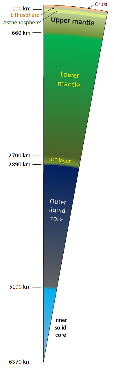
The diagram to the left (Figure 3-1), which is the same as Figure 9.2 in the text, shows the main features of the Earth’s interior.
Figure 3-1 credit: Physical Geology by Steven Earle used under a CC-BY 4.0 international license.
The outermost part is the crust, and at about 50 km thick, it is equivalent in thickness to the skin of an apple.
The next part, and the greatest in volume by far, is the mantle, which makes up 83% of the volume of the Earth. The mantle consists of ferromagnesian silicate minerals and can be divided into five distinct layers: the rigid lithosphere, the nearly-liquid asthenosphere, upper and lower mantle (both solid, but able to flow when subjected to a slow force), and the D” layer, which is also nearly liquid. The overall compositions of these different parts of the mantle are not significantly different, but they have differing physical properties of mineralogy (e.g., although the upper and lower mantle are made of different minerals, they have the same compositions overall).
Although the core-mantle boundary (CMB) is approximately half-way to the centre of the Earth, the volume of the core (16% of the Earth’s volume) is much less than that of the mantle. The core is primarily made of iron. The outer core is liquid, and the inner core, although hotter, is solid because it is under such intense pressure.
As described in Section 9.1, our main source of information about the Earth’s interior is the seismic data from the vast array of seismometers installed at every corner of the planet. Every time a significant earthquake occurs, seismic waves spread through the Earth and are detected at thousands of different locations. All of the detected waves travel though the different parts of the crust, mantle, and core, and their velocities and behaviour provide information about the nature of those various regions of the Earth’s interior.
Before we go any further, it’s important to understand that the waves that pass through the Earth are known as body waves, and that they come in two types: P waves and S waves. The differences between the two are described in the textbook. The critical things to know are that P waves travel faster than S waves, that both types of waves travel faster in hard and strong materials than in soft and weak materials, and that while P waves will pass through a liquid, S waves will not.
The seismic wave velocity diagrams of Figures 9.6 (a) and (b) are based on information from thousands of earthquakes collected at hundreds of seismic stations, which show us how the properties of the materials within the Earth change. The most dramatic changes occur at the core-mantle boundary where the S waves stop altogether, and the P waves slow dramatically because the outer core is liquid. However, other more subtle changes also within the different layers of the mantle. For example, all waves are slowed within the zone called the asthenosphere because the rock is partially molten, and therefore softer and weaker than the rest of the mantle.
Completing Exercise 9.1 will give you some idea of the rate at which P waves travel through the crust.
Section 9.1 in the textbook includes a list of the important behaviours of seismic waves as they pass through the Earth, which is worth repeating here. While reading this list make sure that you can point out these features in Figures 9.6, 9.7, and 9.8:
- Velocities are greater in the mantle than in the crust, which explains the Mohorovičić discontinuity illustrated in Figure 9.7.
- Velocities generally increase with pressure, and therefore with depth, which accounts for the curved-outward pattern of the waves within the Earth as illustrated in Figure 9.8.
- Velocities slow in the area between a 100 km and 250 km depth (called the low-velocity zone, which is equivalent to the asthenosphere) as shown in Figure 9.6.
- Velocities increase dramatically at 660 km depth because of a mineralogical transition.
- Velocities slow in the region just above the core-mantle boundary (known as the D” layer or ultra-low-velocity zone).
- S waves do not pass through the outer part of the core, and P wave velocities are dramatically slowed at this boundary.
- P-wave velocities increase at the boundary between the liquid outer core and the solid inner core.
Complete Exercise 9.2 to help with your understanding of the nature of seismic wave propagation through the Earth.
Section 9.2 describes the pattern of temperature changes within the Earth. As everyone knows, the further down you go into the Earth, the hotter it gets, but the rate of temperature increase is not consistent. The temperature increases quickly in the crust and the uppermost part of the mantle, and then less quickly in the mantle (Figure 9.10). This change is attributed to mixing within the mantle. Like a pot of very thick soup on the stove, the mantle is being heated from below (by the hot core). If mixing was not occurring in the soup pot, the bottom part would get very hot and probably burn, while the top would remain relatively cool. This situation would be reflected by a steep temperature gradient (a relatively flat line in Figure 9.10). If the soup was being stirred continuously, the temperature would be the same throughout (a vertical line in Figure 9.10). The mantle is somewhere between these end points because it is being mixed slowly—not by someone “stirring the pot,” but by convection—so the temperature difference between the bottom and the top is not as great as it would be otherwise. The convection occurring within the mantle (illustrated in Figure 9.12) is a critical component of plate tectonics, which we’ll talk more about later in this unit.
As described at the end of Section 9.2, the sources of heat in the Earth’s interior are mainly leftover heat from the collisions that formed the Earth, and the heat created by natural radioactive decay. The amount of available heat energy is gradually decreasing as the Earth is cooling, but unlike some smaller bodies (Mars and the Moon, for example), enough heat remains to maintain a liquid core, drive mantle convection and plate tectonics, and produce volcanism.
As just mentioned, the Moon and Mars no longer have liquid cores. Go briefly back to Exercise 9.2 and think about what that means for the S wave shadow zones in these bodies.
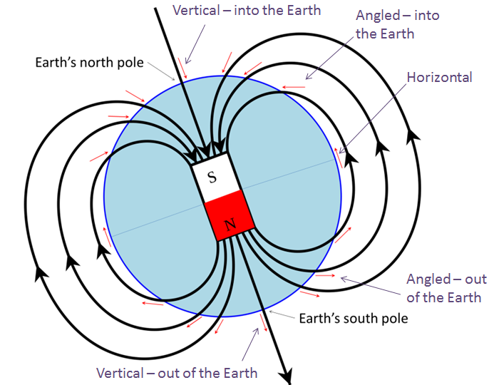
Section 9.3 describes the origins and behaviour of the Earth’s magnetic field. As is summarized in this section, the Earth has a magnetic field because the outer part of the iron-rich core is still liquid and because that material is moving convectively. This field is similar to the typical dipole (two poles, north and south) of a bar magnet as illustrated in Figure 9.13, which means that at the Earth’s surface, the orientation of the magnetic field will vary depending on latitude and longitude. As we’ll see later, this magnetic field has very significant implications for how geologists came to understand plate tectonics.
You can increase your understanding of the orientations of the magnetic field lines by completing Exercise 9.3.
Enlarge
Physical Geology by Steven Earle used under a CC-BY 4.0 international license.
The Earth’s magnetic field is not static. Rather, it varies in intensity, and periodically (on time scales of thousands of years) fades away to almost nothing and then re-establishes itself, sometimes with the opposite polarity (the north arrow of a compass would point to the South Pole). We now understand the chronology of magnetic field reversals, which also has significant implications for how geologists came to understand plate tectonics.
The final section of Chapter 9 includes an overview of isostasy, which we’ve already discussed in the context of metamorphism. The key factor is that the mantle is plastic; it flows or deforms in response to a slowly-applied stress. When a change occurs to the mass of part of the crust—because of mountain building, erosion, glaciation, or deglaciation—the mantle responds by allowing the crust to sink deeper or float higher than before. This process is illustrated in Figures 9.17 and 9.18.
The crust beneath the oceans is compositionally different than that of the continents. Oceanic crust is heavier and sinks lower into the mantle—which is why oceans are below sea level while most parts of the continents extend above sea level.
You can see how this works by completing Exercise 9.4. The differences in the densities of oceanic and continental crust play an important role in how the Earth’s plates interact with each other.
Complete the review questions at the end of Chapter 9, and check your answers in Appendix 2 in the textbook.
3-2 Plate Tectonics
As described in Section 10.1, the concept of continental drift was first conceived by Alfred Wegener just over 100 years ago. In this course, we’re not going to focus on the theories that existed before plate tectonics, but it’s worth reading about continental drift in Section 10.2. As described in Section 10.3, a revolution occurred in geological science between the 1930s and the mid-1960s.
Complete Exercise 10.1 (Section 10.2) to help you understand Wegener’s reasoning.
One of the reasons why Wegener’s theory was largely ignored for 50 years is that it relied on a number of properties of the Earth that simply weren’t understood at the time. For example, Wegener thought that continents moved because they were pushed along over the underlying rocky material, but he couldn’t account for the force that might be doing the pushing, and he couldn’t explain how any known force could overcome the massive amount of friction. Although we now know that the asthenosphere is a relatively weak layer along which plates can slide, and also that convection in the mantle provides some of the push, Wegener and his contemporaries did not have any such knowledge.
Section 10.3 provides a summary of some of the important advances in global geology that were made during the first part of the 20th century. Carefully read that section, making sure you understand the following points:
- In the early 1950s, using magnetic orientation data, it was shown that when ancient rocks in Europe were deposited, the magnetic pole positions were different than they are now. First, it was thought that this was the result of “polar wandering,” but later geologists realized that this phenomenon was more consistent with the concept of moving continents (Figure 10.6).
- During the first half of the 20th century, our understanding of the topography of the sea floor increased dramatically. This knowledge led to the discovery of mid-ocean ridges, deep trenches along continental edges, and chains of seamounts (Figure 10.8). Although these features were not fully understood at first, we now know that they are respectively related to sea-floor spreading at divergent boundaries, subduction at convergent boundaries, and volcanism where a plate moves slowly over a mantle-plume.
- The application of seismic sounding over wide areas of the sea floor has enabled geologists to map differences in the thickness of sea-floor sediments, and to see that while sediments are thick in most parts of the ocean, they are very thin in areas near to the mid-ocean ridges (Figure 10.9). We now know that these differences can be explained by the fact that the sea floor in these areas is very young and not enough time has passed for thick sediments to accumulate.
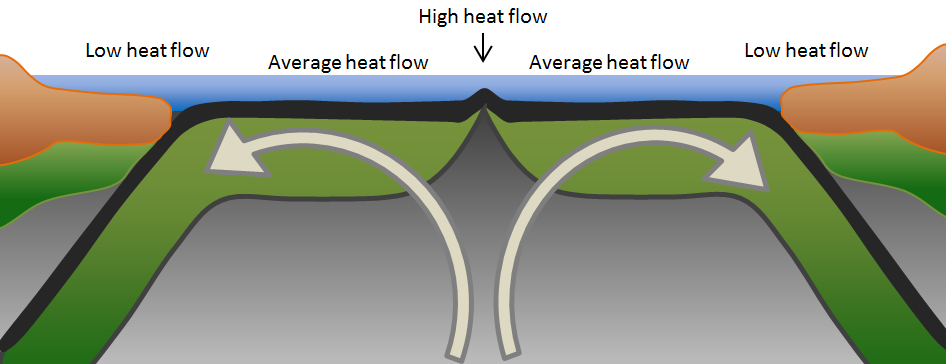
- In the 1950s, measurements of heat flow through the sea-floor showed that a greater than average amount of heat was produced in ridge areas than elsewhere, and that less heat was produced in areas close to the trenches. This phenomenon was interpreted to be the existence of convection within the mantle as is shown in Figure 3-3.
Enlarge
© Steven Earle. Used with permission.
- The development of networks of seismic stations, between the 1930s and the 1950s, enabled a relatively precise positioning (location and depth) of earthquake locations. It was shown that while most significant earthquakes are shallow, they get progressively deeper inshore from the oceanic trenches as is illustrated in Figure 10.10.
- In the 1950s and 1960s, the acquisition of magnetic data from the oceans showed a complex pattern of high and low magnetic regions in what was known to be rock of a very consistent basaltic composition (Figure 10.11). Although not understood at first, in 1963, Vine, Matthews, and Morely argued that these patterns were a result of new sea-floor crust being formed during times of normal and reversed magnetism.
- Also in 1963, geologists found that the ages of the Hawaiian Islands increased systematically with distance from the still-active volcanoes on the big island, which led to the concept that a stationary hot spot (mantle plume) existed beneath the big island, and that the Pacific sea-floor crust was moving over top of that source of volcanism (Figure 10.13).
- Finally, in 1965, a new type of fault—called a transform fault—was described and explained as being caused by moving plates. Transform faults are common along spreading ridges (Figure 10.15), but also are present on land, where they are associated with significant earthquake risks.
In Exercise 10.2, you can see for yourself how the ages of the Hawaiian islands vary with location.
Completing Exercise 10.3 should help you to understand transform faults, and also the process by which the sea floor crust becomes varyingly magnetized.
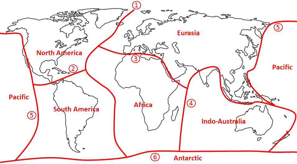
The theory of plate tectonics finally became widely accepted in the mid-1960s, mostly as a result of the compelling evidence of Vine, Matthews, and Morely, and the work of Tuzo Wilson on hot spots and transform faults. Wilson also played an important role in mapping the boundaries between plates on the Earth’s surface, showing how these plates were moving, and describing the various processes that occur at different types of plate boundaries. Figure 10.16 is a modern map of the plates, their directions and rates of motion, and the types of boundaries between them. More than 20 different plates exist, and you should know the names and approximate extents of the seven major ones. A simple way to learn these names and locations is to roughly draw in their boundaries as shown on Figure 3-4. Start with (1) a curvy line down the middle of the Atlantic Ocean. Separate South America from North America (2), and Eurasia from Africa (3). Draw a boundary through the Indian Ocean and separate India and Australia from Asia (4). Draw a line generally around the Pacific Ocean (5), and finally draw a line all the way around Antarctica (6).
Enlarge
© Steven Earle. Used with permission.
Exercise: Without looking at Figure 3-4, draw in the boundaries of the seven major plates on the following map. (If needed, follow the instructions beneath the map.) After you’re done, refer to Figure 10.16 in the textbook and add arrows to show the approximate plate motions.
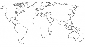
Start with a curvy line down the middle of the Atlantic Ocean. Separate South America from North America, and Eurasia from Africa. Draw a boundary through the Indian Ocean, and separate India and Australia from Asia. Draw a line generally around the Pacific Ocean, and finally draw a line all the way around Antarctica.
To understand plate tectonics, it’s important to know what a plate is. As shown in Figure 10.17, tectonic plates are not only comprised of continental or oceanic crust, but also include the underlying lithospheric (“rigid”) part of the mantle. This package of crust plus lithospheric mantle—which is about 100 km thick on average—is known as the lithosphere, which slides across the top of the asthenosphere when a plate moves.
Section 10.4 describes the processes that occur at plate boundaries, starting with divergent (spreading) boundaries where new oceanic crust is made. The key to this process is the convection-related upwelling of hot mantle rock, and the decompression melting of some (about 10%) of that rock within 60 km of the sea floor (Figure 10.18). Figure 10.19 provides a summary of the types of rocks produced in this environment, which include gabbro at depth, mafic dykes in the middle, and pillow basalts near to the sea floor.
Figure 10.20 illustrates the process that is thought to be responsible for the rifting of continents and the formation of new spreading boundaries. Please make sure that you understand this process.
Figures 10.21, 10.22, and 10.23 show two plates moving towards each other at a convergent boundary. Before going any further with this, you need to be aware that tectonic plates never have a gap between them, since they are moving towards each other and then eventually collide. Convergent boundaries can form within plates, and are most likely to occur at the ocean-continent interface within a plate that includes both oceanic and continental crust. For example, the North America Plate includes both the continental crust of North America and the oceanic crust of the western Atlantic Ocean. Along the eastern coast of North America, a transition exists between the continental and oceanic crust as depicted in Figure 3-5 (left). Both parts are being pushed to the west by spreading along the mid-Atlantic ridge, which is called a passive margin. At some time in the distant future, the oceanic and continental lithospheres could separate, and subduction could begin along this boundary (Figure 3-5 right). This is likely to be due to the accumulation of sediment along the boundary as is described in more detail towards the end of Section 10.4.
Enlarge
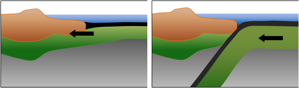
© Steven Earle. Used with permission.
In Section 10.4, read carefully through the material on convergent boundaries. Some of the important points are that water from the subducting crust contributes to melting in the overlying hot mantle rock, and that the compressive stress of convergence leads to faulting and deformation, not only in the continental crust, as is shown in Figure 10.22, but also in the oceanic crust on both sides of the boundary.
As already mentioned, most transform faults exist at spreading ridges where they form the boundaries between offset ridge segments. They also form the boundaries between plates as is illustrated in Figure 3-6. In this figure, the two plates have been highlighted in different colours, and you can see how the ridge segments (double white lines) form the plate boundary at some locations, whereas the transform faults (red lines) form the plate boundary at other locations. The white lines that extend out on either side of the ridge segments are called fracture zones. These zones are not plate boundaries, and providing the rates of spreading on the various ridge segments are similar, no relative motion (i.e., no faulting) occurs along these lines.
Enlarge
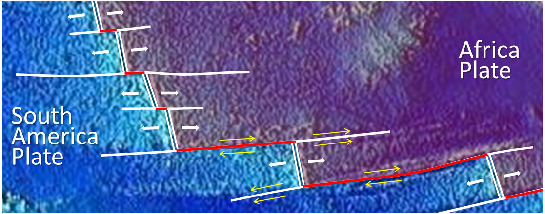
Physical Geology by Steven Earle used under a CC-BY 4.0 international license.
In some cases, transform boundaries cut across continents, for example, the San Andreas Fault. All transform faults are characterized by motion that is essentially horizontal.
Completing Exercise 10.4 will contribute to your understanding of transform boundaries.
The remaining part of Section 10.4 includes a summary of some relatively recent and near-future expected changes in the Earth’s tectonic plate configuration. It also includes a discussion of the Wilson Cycle and a more complete description of how a passive ocean-continent margin can change into a subduction boundary (Figure 10.26).
Test your recollection of plate names, and your understanding of plate boundaries by completing Exercise 10.5.
Section 10.5 includes a brief discussion of the mechanisms for plate motion. Although we’ve said all along that convection in the mantle is the critical driver of plate tectonics, some related phenomena exist—including the gravitational push away from the elevated ridge areas (ridge push) and the gravitational pull of subducting oceanic crust (slab pull)—that contribute to plate motion. The three processes essential to the movement of plates are summarized in Figure 10.29.
Before moving on to Section 3-3 on earthquakes, answer the review questions at the end of Chapter 10.
3-3 Earthquakes
As noted in Section 11.1, an “earthquake is the shaking caused by the rupture (breaking) and subsequent displacement of rocks (one body of rock moving with respect to another) beneath Earth’s surface.” Before a body of rock breaks, it has to be strained (deformed) (Figure 11.2), and in almost all cases, that strain is caused by the relative motion at plate boundaries. Where two plates are in contact with one another, the rocks on either side don’t typically slide smoothly past each other; instead, they stick along the boundary and then slowly deform elastically. Although the amount of deformation that the rock can withstand depends on its strength, all rock that is progressively strained will eventually be unable to handle the strain, and will break.
Earthquakes do not occur at a single point within the crust, nor at a single moment in time. The displacement happens over an area called the rupture surface (Figure 11.3), and is greatest near to the middle of that surface and least towards the margins. The area of the rupture surface and the average amount of displacement determine the size (magnitude) of an earthquake. The displacement within a rupture surface occurs over a period of seconds (or even minutes if it’s a very large quake) and is characterized by a series of small earthquakes (immediate aftershocks), all of which are related to each other by the process known as stress transfer, which means that the reduction in stress in one area of the rupture surface actually adds to the stress elsewhere (see Figure 11.6). Understanding stress transfer and aftershocks is critical to understanding earthquakes, so carefully read that part of Section 11.1, including the material on episodic tremor and slip.
As described in Section 11.2, and shown in Figure 11.7, the relationship between plate boundaries and earthquakes is very strong. The vast majority of earthquakes occur within a few tens of kilometres of plate boundaries, and in some cases, on the boundary plane or a nearby structure (a fault) that is associated with the boundary. Figure 3-7 shows the known earthquake-producing faults in the area around San Francisco. The San Andreas Fault, which defines the boundary between the Pacific and North America Plates, has been responsible for many large quakes (including the devastating 1906 San Francisco earthquake and the damaging 1989 Loma Prieta earthquake), but other faults in the region also have caused significant quakes, and the greatest risk over the next 20 years is predicted to be the Hayward and Rodgers Creek Faults.
Enlarge
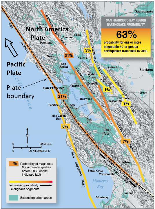
Adapted from: USGS. 2008 Bay area earthquake probabilities [Digital image]. Earthquake Hazard Program. U.S. Geological Survey.
As shown in Figure 11.8, most earthquakes in the vicinity of spreading ridges actually occur on the transform faults between ridge segments, rather than on the ridge itself.
Figure 11.10 shows a typical distribution of earthquakes associated with the subduction zone of a convergent boundary. Again, lots of earthquakes occur tens to even hundreds of kilometres from the actual plate boundary, but when a very large earthquake happens (like this 2009 example), the shocks related are mostly confined to the upper (cooler) part of the plate boundary.
As is shown in Figure 11.11, southern and central Asia have a vast region of occurring earthquakes where the India Plate is being forced into the Eurasia Plate. It is evident that the rock over a very wide area is being strained by this continent-continent convergence.
Working on the questions in Exercise 11.1 will help you to understand the earthquakes associated with subduction and transform boundaries in western Canada.
In Section 11.3, we look at some of the ways of measuring earthquakes. The magnitude of an earthquake is an expression of how much energy was released, and is most often determined using seismic data. Be sure to review the material in the textbook on body waves and surface waves. Many methods are available to estimate magnitude—summarized in Table 11.1—but each earthquake has only one actual magnitude.
In Exercise 11.2, you can play with a tool that enables you to estimate the moment magnitude of a number of different earthquakes using values for the length and width of the rupture surface and the amount of displacement. The last question asks you to use this tool to estimate the length, width, and displacement values for a M10 earthquake. This estimation will help you to understand why the size of earthquakes is limited on Earth.
Exercise: Think about what necessary characteristics a planet would need for earthquakes to occur at a magnitude higher than 10.
As described in Section 11.3, an increase of 1 unit on the magnitude scale is equivalent to a 32-fold difference in the amount of energy released. Very large earthquakes (magnitude 8 or higher) release millions of times more energy than very small ones (magnitude 2 or less).
Exercise: The December 2015 earthquake in the Saanich region of British Columbia had a magnitude of 4.7. The October 2012 earthquake off the coast of Haida Gwaii had a magnitude of 7.7. How many times more energy was released by the Haida Gwaii earthquake than the Saanich earthquake?
The other way of measuring earthquakes is to assess what people felt, and what type of damage was done. This is known as intensity, which is based on a descriptive scale (the modified Mercalli Intensity Scale in Table 11.2) that someone can use to assign a value based on her/his experience or his/her assessment of damage done to buildings. Unlike magnitude, intensity estimates for a single earthquake can vary widely, depending first on the distance of the observation site to the earthquake, and second on the type of geological material underlying the site. As noted in the textbook, shaking tends to be greatest in areas underlain by soft unconsolidated sediments, such as former lake sediments, fine-grained river sediments, or glacial sediments. These weak materials tend to have natural vibrational frequencies in the 2 to 3 second range (as compared to much less than 1 second for solid rock). This range of frequencies matches the frequency of the powerful body waves of earthquakes, which causes a resonant amplification of the shaking in the weak materials.
In Exercise 11.3, you can try your hand at assigning intensity values to actual observations made in 2001 in various parts of Nanaimo, BC, of an earthquake south of Seattle. You’ll find that the experiences of people were quite different, although they all were almost exactly the same distance (~250 km) from the quake. Think about why these differences occurred.
Creating intensity maps, like the one in Figure 11.16, is very useful because it provides us with some knowledge about which parts of a region are especially susceptible to earthquake shaking.
Some of the risks associated with large earthquakes are summarized in Section 11.4. Most earthquake damage is done to buildings, especially those with rigid rather than flexible frameworks. Wood-frame buildings, for example, tend to perform much better during seismic shaking than brick or concrete buildings. Another important principle of earthquake resistant design is to construct buildings and other structures that don’t resonate in the 2 to 3 second range. This type of construction often can be achieved by using diagonal bracing as shown in Figure 3-8 on a building in Berkeley California close to the Hayward Fault.
Enlarge
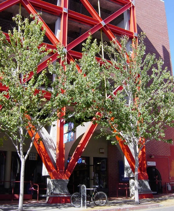
Leonard G. (2004). Exterior general reenforcement of an existing garage structure with street level shops [Digital image]. Wikimedia Commons. Retrieved from: https://commons.wikimedia.org/wiki/File:ExteriorShearTrussTwo.jpg
As you read through Section 11.4, you’ll see that time and time again the greatest damage caused by earthquakes occurs in areas underlain by water-saturated soft sediments, where an amplification of the shaking and liquefaction of the material are both possible. In earthquake-prone regions, geological mapping to identify substrate characteristics is an important aspect of risk mitigation. Where no other options exist but to build on soft sediments—such as in the Fraser Delta area south of Vancouver—steps can be taken to compress and strengthen the material prior to construction, or to build on pilings that have been driven deep into the subsurface.
To get a better understanding of harmonic amplification and liquefaction, complete Exercise 11.4.
The other main risk from earthquakes is the generation of tsunami. Tsunami were primarily responsible for most of the 280,000 deaths in one of the Earth’s deadliest earthquakes—Sumatra, 2004—and for most of the tens of billions of dollars in damage in one of the Earth’s costliest earthquakes—Tohoku Japan, 2011. Tsunami are almost exclusively generated by large (M >8) subduction-related earthquakes, since these quakes typically involve vertical displacement of the sea floor by up to several metres over thousands of square kilometres.
It has long been a dream of seismologists and public safety officials to be able to accurately predict earthquakes so to minimize damage and casualties. However, as summarized in Section 11.5, we are not close to that goal. Although some researchers have claimed limited success by detecting changes in some parameters prior to some earthquakes, there appears to be no precursor signal or observation that is consistently found prior to all earthquakes. To be successful, earthquake predictors need to be accurate most of the time, not just some of the time. People tend to quickly become very skeptical when presented with repeated false alarms. The biggest blow to earthquake prediction was delivered at Parkfield California in 2004, where hundreds of sensors and detectors of all imaginable types failed to record any prior signal of the M6 earthquake.
One important relatively recent advance is in the field of very fast automatic sensing and the characterization of earthquakes based on their P wave signal. In areas with seismometer networks close to the expected locations of earthquakes, rapid detection can provide warnings that an earthquake has just happened (as distinct from a prediction that it is about to happen). Ocean Networks Canada, an initiative of the University of Victoria, has installed an ocean-floor observatory network up to 200 km offshore from the west coast of Vancouver Island (Figure 3-9). Included in this network are several seismometers that are capable of detecting earthquakes as they happen. If the P wave signals from an earthquake are processed automatically, the information about its magnitude and location can be sent to emergency officials and utilities within less than a second, which would provide warning times of 60 to 70 seconds for populated regions on eastern Vancouver Island (e.g., Nanaimo and Victoria) and over 80 seconds for the Metro Vancouver region prior to the arrival of the first damaging S waves. That is plenty of time for utilities to shut down electrical circuits or close pipeline valves, and also would make it possible for many individuals to get to safer places.
Exercise: Try this out for yourself. Set a timer for 70 seconds and then see what you can do to ensure your own safety from an earthquake in that amount of time. It might mean moving to a safe place within a building, or getting outside and well away from buildings. Or it could mean not driving onto a bridge or quickly driving out of tunnel. If you’re near to the shore, it also would give you time (at least 30 minutes) to get to higher ground, out of the way of a potential tsunami.
Enlarge
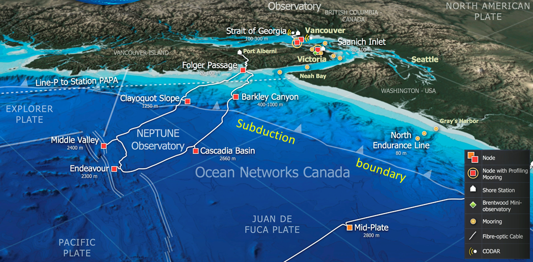
Adapted from Ocean Networks Canada. (2013). Ocean science in the Northeast Pacific. Flickr. Retrieved from: https://flic.kr/p/i5UVCv .
While we cannot predict earthquakes, we increasingly have good knowledge about areas that are at risk, and we can start to express that risk in terms of probabilities, as has been done in the San Francisco area by the US Geological Survey (Figure 3-7). If we know the risks in a certain area, we can start to prepare by creating and enforcing strong building codes, retrofitting important buildings such as schools, making public and personal emergency plans, and educating the public.
Please answer the review questions at the end of Chapter 11, and check your answers in Appendix 2 in the textbook.
This completes the notes for Unit 3.
Note if you are a registered student: If you haven’t already done so, now is the time to start working on Assignment 3 (go to “Assignments” on the course Home Page). You should find most of what you need to complete the assignment within these unit notes and Chapters 9 to 11 of your textbook, but you might also need to refer to other sources of information.